Wildcard Match: Robust KV Cache Management for LLM Serving under Output Token Length Uncertainty

一、论文概述

项目	内容
标题	Robust KV Cache Management for LLM Serving under Output Token Length Uncertainty
作者	Jiaming Cheng, Duong The Do, Duong Tung Nguyen
机构	—
论文	arXiv:2607.16892
代码	— (未开源)
发布	2026-07-18 (Globecom 投稿)

核心贡献：

1. 提出一个鲁棒 KV cache 管理框架，联合优化 GPU 并行配置、每请求类 KV cache 预留、异构服务组间请求路由和前缀缓存
2. 将输出 token 长度不确定性建模为 Wasserstein 分布鲁棒优化（DRO）问题，推导了可处理的有限维 reformulation（MIBLP）
3. 揭示了最优预留策略的临界分位数结构（critical fractile structure）——自动适应不同 preemption 和 memory cost 场景，无需手动调参
4. 设计了可扩展的块坐标下降算法 BCD-DRO，支持周期性 re-optimization
5. 在 BurstGPT、Azure 和 ShareGPT 三个生产级 trace 上的评估表明：相比固定分位数基线最高降低 56% 成本，同时保持竞争性 P99 延迟

二、核心思想

问题定义

KV cache 内存是现代 LLM serving 系统的主要瓶颈。根本挑战在于：KV cache 必须在请求到达时预留，而输出 token 长度直到生成完成才可知。

• 预留不足 → 触发 preemption（终止请求并重新计算），产生显著 overhead
• 预留过多 → 浪费内存，降低 throughput

这形成了一个核心的权衡：memory efficiency vs. preemption risk。

具体挑战：

1. 工作负载异质性：不同应用类（chat、code generation、QA）的输出长度差异可达几个数量级
2. 输出长度不确定性：同一请求类内的输出长度波动很大
3. 共享 GPU 内存：多个请求类竞争有限的 KV cache 容量
4. 分布漂移：训练期间的历史数据与线上实际分布可能存在偏移

解决方案概述

WAR 的核心方法：将 KV cache 预留建模为一个联合优化问题，包含四个控制变量：

1. GPU 并行配置 $z_k$：每个配置部署多少个 serving group
2. KV cache 预留 $r_i$：每类请求预留多少 token
3. 请求路由 $\pi_{i,k}$：每类请求路由到哪个配置
4. 前缀缓存 $\delta_{i,k}$：是否缓存某类的共享前缀

通过 Wasserstein DRO 处理输出长度不确定性和工作负载分布漂移。

三、技术架构

整体框架

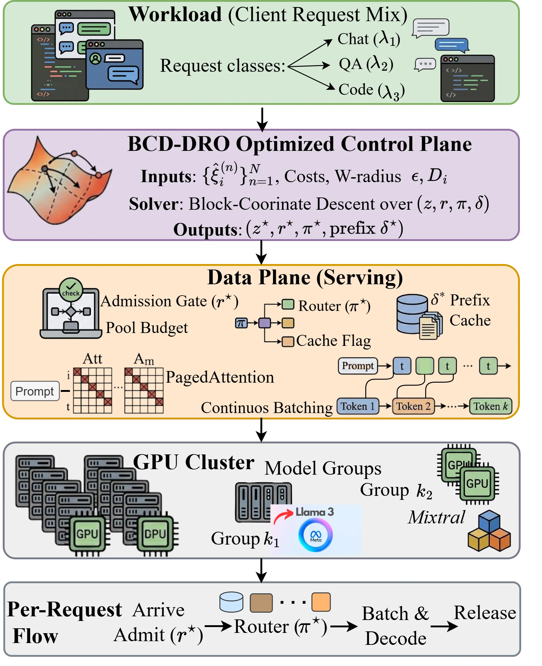
BCD-DRO 是一个控制平面策略，接收历史样本、成本参数和 Wasserstein 半径，在每个 re-optimization tick 产出四个控制变量 $(z^*, r^*, \pi^*, \delta^*)$。数据平面（PagedAttention、continuous batching、可选 P/D split）直接使用这些变量，无需修改。GPU 集群执行 decoding，遥测反馈关闭滚动时域循环。

系统模型

集群配置

考虑一个拥有 $J$ 个 GPU 的 LLM 服务提供商。将 GPU 划分为 serving groups，每组使用特定的并行配置。令 $\mathcal{K}$ 为候选配置集合，每个 $k \in \mathcal{K}$ 指定 tensor parallelism degree $\tau_k$ 和 pipeline parallelism degree $p_k$，每组消耗 $\tau_k p_k$ 个 GPU。每种配置有派生的 KV cache 容量 $M_k$（token 数）和有效 compute/bandwidth $(C_k, B_k)$。

请求类

请求根据应用类型分为 $i \in \mathcal{I}$ 个类（chat、code generation、QA）。每类 $i$ 有：

• 到达率 $\lambda_i$
• 输入长度 $L_{\text{in}}^i$（已知）
• 共享前缀 $L_{\text{pre}}^i$（可缓存）
• 延迟 SLO $D_i$
• 输出长度 $\xi_i$（生成完成前未知）

服务时间

LLM 推理包括 compute-bound prefill 和 memory-bandwidth-bound decode 两个阶段。类 $i$ 在配置 $k$ 上的期望服务时间为：

$$T_{i,k} = \underbrace{\frac{p_k \alpha L_{\text{in}}^i}{C_k}}_{\text{prefill + bubble}} + \underbrace{\frac{\beta \mathbb{E}[\xi_i]}{B_k}}_{\text{decode}} + \underbrace{N_L \tau_k t_{\text{ar}}}_{\text{comm.}} \tag{1}$$

其中 $\alpha, \beta$ 是模型特定常数，$N_L$ 是层数，$t_{\text{ar}}$ 是 all-reduce 延迟。注意服务时间使用 $\mathbb{E}[\xi_i]$ 而非不确定的实现值 $\xi_i$，因为 throughput 是聚合指标——根据大数定律，并发请求间的波动会平均化。

决策变量

算子联合优化四个决策（在观察到实际输出长度之前做出）：

变量	符号	含义
配置部署	$z_k \in \mathbb{Z}_+$	使用配置 $k$ 的 serving group 数量
KV cache 预留	$r_i \in [L_{\text{in}}^i, L_{\text{in}}^i + L_{\text{max}}^i]$	每类 $i$ 请求预留的 KV cache tokens
请求路由	$\pi_{i,k} \geq 0$	类 $i$ 请求中路由到配置 $k$ 的比例
前缀缓存	$\delta_{i,k} \in \{0, 1\}$	是否在配置 $k$ 上缓存类 $i$ 的共享前缀

被拒绝的部分满足 $\pi_{i,0} = 1 - \sum_k \pi_{i,k}$。

成本结构

Preemption Cost（预留不足）

当预留的 KV cache 不足以容纳生成的 tokens 时发生 preemption：$L_{\text{in}}^i + \xi_i > r_i$。此时成本为：

$$C_{\text{preempt}} = c_p \cdot (L_{\text{in}}^i + \xi_i - r_i)^+ \tag{2}$$

Waste Cost（预留过多）

当预留的 KV cache 超过实际使用时，未使用的内存无法被其他请求利用：

$$C_{\text{waste}} = c_w \cdot (r_i - L_{\text{in}}^i - \xi_i)^+ \tag{3}$$

Cost Ratio

预emption 和 waste 项共同捕捉了一个根本权衡：预留太少导致昂贵的重计算，预留太多减少并发服务能力。成本比 $\rho = c_p/c_w$ 编码了 under- 和 over-reservation 之间的不对称性，直接决定最优预留分位数。

总成本

每类 $i$ 到达的期望成本结合随机和确定性分量：

$$Q_i = \underbrace{a_i \cdot \mathbb{E}[c_p(\cdot)^+ + c_w(\cdot)^+]}_{\text{preempt/waste (admitted)}} + \underbrace{C_{\text{gpu}} + C_{\text{slo}} + C_{\text{rej}}}_{\text{resource, SLO, rejection}} \tag{4}$$

其中 $a_i = \sum_k \pi_{i,k}$ 是 admission probability。

完整优化问题

联合优化问题：

$$\min_{z, r, \pi, \delta, s} \sum_{i \in \mathcal{I}} \lambda_i \left[ a_i \sup_{P \in \mathcal{P}_\varepsilon^i} \mathbb{E}_P[Q_i^{\text{stoch}}] + Q_i^{\text{det}} \right] \tag{6a}$$

s.t.

$$\sum_{k \in \mathcal{K}} z_k (\tau_k p_k) \leq J \tag{6b}$$ $$\pi_{i,k} \leq z_k, \quad \forall i \in \mathcal{I}, k \in \mathcal{K} \tag{6c}$$ $$\sum_{k \in \mathcal{K}} \pi_{i,k} + \pi_{i,0} = 1, \quad \forall i \in \mathcal{I} \tag{6d}$$ $$(1+\kappa) \sum_{i \in \mathcal{I}} u_{i,k} \pi_{i,k} \leq \sum_{i \in \mathcal{I}} z_k \tilde{r}_{i,k} \tag{6e}$$ $$s_i \geq \sum_{k \in \mathcal{K}} \pi_{i,k}(W_k + T_{i,k}) - a_i D_i, \quad s_i \geq 0 \tag{6f}$$

约束解释：

• (6b) GPU 预算：所有 serving groups 的总 GPU 消耗不超过 $J$
• (6c) 路由一致性：只能路由到已部署的配置
• (6d) 路由概率：每类请求要么路由到某配置，要么被拒绝
• (6e) 内存容量：关键约束，通过 Little’s law 将预留与 throughput 耦合
• (6f) SLO 约束：期望响应时间（等待 $W_k$ + 服务 $T_{i,k}$）必须满足延迟目标 $D_i$

其中 $W_k$ 来自 Pollaczek-Khinchin 公式：

$$W_k = \frac{\alpha_\lambda \bar{T}_k}{2(1-u_k)} \left( \frac{\alpha_\lambda^2 + \sigma_{T,k}^2 / \bar{T}_k^2}{2} + (1+u_k) \right) \tag{7}$$

DRO formulations

输出长度 $\xi_i$ 遵循未知分布 $P^i$。采用 Wasserstein 歧义集：

$$\mathcal{P}_\varepsilon^i = \left\{ P^i : W_1(P^i, \hat{P}_N^i) \leq \varepsilon \right\} \tag{5}$$

其中 $W_1$ 是 1-Wasserstein 距离，$\varepsilon \geq 0$ 控制鲁棒性。

可处理 reformulation（Proposition IV.1）

通过 Kantorovich duality，无限维 DRO 目标等价于有限维 MIBLP：

\begin{aligned} \min_{z,r,\pi,\delta,\gamma,\theta,s}~& \sum_{i \in \mathcal{I}} \lambda_i \left[ \sum_{k \in \mathcal{K}} \pi_{i,k} \left( \gamma_i \varepsilon + \frac{1}{N} \sum_{n=1}^N \theta_{i,n} \right) + Q_i^{\text{det}} \right] \tag{8a} \\ \text{s.t.}~&(6b)\text{--}(6f) \tag{8b} \\ \theta_{i,n} &\geq c_p(\hat{\xi}_i^{(n)} + L_{\text{in}}^i - r_i), \quad \forall i, n \tag{8c} \\ \theta_{i,n} &\geq c_w(r_i - L_{\text{in}}^i - \hat{\xi}_i^{(n)}), \quad \forall i, n \tag{8d} \\ \theta_{i,n} &\geq c_p(L_{\text{max}}^i + L_{\text{in}}^i - r_i) - \gamma_i(L_{\text{max}}^i - \hat{\xi}_i^{(n)}), \quad \forall i, n \tag{8e} \\ \theta_{i,n} &\geq c_w(r_i - L_{\text{in}}^i) - \gamma_i \hat{\xi}_i^{(n)}, \quad \forall i, n \tag{8f} \\ \gamma_i &\geq 0, \quad \theta_{i,n} \geq 0, \quad \forall i, n \tag{8g} \end{aligned}

其中 $\gamma_i$ 是 Wasserstein 约束的对偶变量，$\theta_{i,n}$ 是每个 sample $n$ 的辅助变量。

对偶变量解释（Remark 1）： $\gamma_i$ 作为 transportation cost penalty：大的 $\gamma_i$ 使 worst-case distribution 接近 empirical data，小的 $\gamma_i$ 允许质量向极端值（0 或 $L_{\text{max}}$）转移。

临界分位数结构（Proposition IV.2）

这是核心理论结果。考虑固定路由下类 $i$ 的预留子问题。令 $\rho = c_p/c_w$ 为 cost ratio。最优预留 $r_i^*$ 满足：

$$r_i^* = L_{\text{in}}^i + F_i^{-1}\left( \frac{\rho}{\rho+1} \right) \tag{9}$$

其中 $F_i$ 是 DRO 最坏情况下输出长度的累积分布函数。

证明思路： 定义 $\eta = r_i - L_{\text{in}}^i$ 为 output length uncertainty 的 buffer。随机成本为 $Q_i^{\text{stoch}}(\eta, \xi) = c_p(\xi-\eta)^+ + c_w(\eta-\xi)^+$。对期望成本关于 $\eta$ 求导：

$$\frac{\partial}{\partial\eta} \mathbb{E}[Q_i^{\text{stoch}}] = -c_p \cdot \Pr(\xi > \eta) + c_w \cdot \Pr(\xi \leq \eta) \tag{10a}$$ $$= -c_p(1-F(\eta)) + c_w F(\eta) = (c_p+c_w)F(\eta) - c_p \tag{10b}$$

令为零得 $F(\eta^*) = c_p/(c_p+c_w) = \rho/(\rho+1)$。因此 $\eta^* = F^{-1}(\rho/(\rho+1))$，给出 $r_i^* = L_{\text{in}}^i + F_i^{-1}(\rho/(\rho+1))$。

临界分位数（Remark 3）： 阈值分位数 $q^* = \rho/(\rho+1)$ 是 critical fractile——增加预留的边际成本等于避免 preemption 的边际收益。随着 $\rho$ 增大（preemption 更昂贵），最优分位数上升，导致更保守的预留。这是经典的 newsvendor critical ratio 的分布鲁棒形式。

Key Takeaway 1： 临界分位数 $q^* = \rho/(\rho+1)$ 是 DRO 的”自调节旋钮”——系统在经济上自动变得保守（preemption 昂贵时）或激进（over-reservation 成本高时），消除了手动分位数调优的需求。

BCD-DRO 算法（Proposition IV.3）

MIBLP 可通过全局求解器精确求解，但对实时部署代价高昂。问题具有 block 结构：连续路由/预留变量 $(r, \pi, \gamma, \theta)$ 在其它 block 固定时与二元缓存决策 $\delta_{i,k}$ 和整数配置 $z_k$ 解耦。这激励了一个块坐标下降（BCD）算法：

Algorithm 1: BCD-DRO Algorithm

0: Samples {ξ̂_i^(n)}, radius ε, configurations K
0: Solution (z*, r*, π*, δ*)
1: Initialize z^(0), δ^(0) ← 0, γ_i^(0) ← c_p, r_i^(0) ← L_in^i + E[ξ_i]
2: for t = 1, ..., T_max do
3:   Block 1: Alternate LP1 (fix γ,θ,r; optimize π) and LP2 (fix π; optimize r,γ,θ) until convergence
4:   Block 2: δ_i,k^(t) ← 1[u_i,k π_i,k / z_k > 1]
5:   Block 3: z^(t) ← arg min_{z∈Z} Obj(z, r, π, δ^(t))
6:   if (z^(t), δ^(t)) = (z^(t-1), δ^(t-1)) then break
7: end for
10: return (z^(t), r, π, δ^(t))

收敛性（Proposition IV.3）： 算法在有限迭代内终止，返回 blockwise optimal solution——即没有单个 block 可以在其它 block 固定时改进目标。

复杂度： offline phase 求解一系列 LPs；runtime scale 与 request classes、samples 和 configuration candidates 的数量相关。online phase 是 $O(1)$ per request：只需采样 routing decision 并应用 precomputed reservation。

Key Takeaway 2： BCD-DRO 的 decomposition 使得在单体求解器失败的 production-scale 部署成为可能，将 KV cache 预留从静态离线决策转变为自适应在线策略。

四、核心创新

创新点	说明	理论/实验依据
Wasserstein DRO for KV cache	将 KV cache 预留建模为 Wasserstein DRO 问题	Eq. (5)-(9)：处理输出长度不确定性和分布漂移
Critical fractile structure	推导出最优预留的 closed-form 分位数结构	Prop. IV.2：$q^* = \rho/(\rho+1)$，自适应 cost regime
Joint 4-knob optimization	联合优化 GPU 配置、预留、路由、前缀缓存	Eq. (6)：唯一的 co-optimize 所有四 knob 的方法
BCD-DRO 分解算法	将 MIBLP 分解为三个 block 交替求解	Alg. 1：production-scale 部署可行性
Rolling horizon adaptation	周期性 re-optimization 跟踪工作负载演化	Fig. 5(a)：static vs rolling horizon 对比

五、代码实现分析

实现基础：

• BCD-DRO 作为一个 control-plane policy 实现
• 数据平面（PagedAttention、continuous batching、可选 P/D split）无需修改即可消费 BCD-DRO 的控制变量
• 支持 periodic re-optimization 以跟踪工作负载演化

关键模块：

1. MIBLP Solver：求解 reformulated 问题的精确求解器（小规模验证用）
2. BCD-DRO Engine：块坐标下降求解器，支持 production-scale 部署
3. Scenario Simulator：trace-driven simulator，用于 offline policy evaluation
4. Queueing Model：基于 Pollaczek-Khinchin 公式的等待时间和容量建模

硬件要求：

• 模拟环境：$J=8$ A100-80GB GPUs serving 70B model
• 生产评估：48-GPU cluster

六、实验结果

实验设置

配置项	值
模拟硬件	$J=8$ A100-80GB GPUs, serving 70B model
并行配置	$k_1$: (TP=2,PP=1), $k_2$: (TP=4,PP=1), $k_3$: (TP=2,PP=2), $k_4$: (TP=4,PP=2)
Trace 数据集	BurstGPT (1.4M req, 61 days), Azure LLM 2024 (44M req, 7 days), ShareGPT (368K req)
成本参数	$c_p/c_w = 10$, $c_{\text{slo}}/c_w = 5$, $c_{\text{rej}}/c_w = 5000$, $\kappa = 0.2$
Wasserstein 半径	$\varepsilon = 0.15 \cdot \mathbb{E}[\xi_i]$
Baselines	Max, Mean, P90, P95, P99, SAA ($\varepsilon=0$), LP+$k\sigma$

DRO vs Fixed-Quantile Baselines

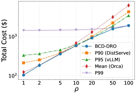
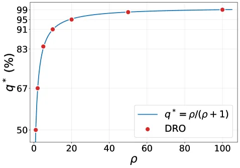
关键发现：

• 没有单一固定分位数启发式在所有 cost regime 下是最优的
• 由 Proposition IV.2，每个固定分位数 baseline 仅在其分位数匹配 critical fractile $q^* = \rho/(\rho+1)$ 时才最优
• Fig. 2(b) 确认 DRO 的 empirical quantile 精确追踪理论公式

Table II: DRO vs baselines across application scenarios

Scenario	$\rho$	DRO	P90	P95	DRO Gain [vs P90, vs P95]
Batch	2	184	255	365	28–50%
Async API	5	360	380	459	5–22%
User-facing	10	587	588	617	0–5%
Latency-sensitive	20	931	1003	931	0–7%
Critical	50	1575	2250	1875	16–30%
Real-time	100	1919	4328	3448	44–56%

关键发现： DRO gain 随 $\rho$ 增大而增长。Real-time 场景（$\rho=100$）下 DRO 比 P90 低 56% 成本。

Table IV: Cost across three cost-ratio regimes

Method	Cost ρ=2	Cost ρ=10	Cost ρ=100	P99 (s) @ ρ=10	SLO viol. @ ρ=10
DRO (ours)	1,270	3,083	4,807	11.47	15.6%
P90	1,852	3,095	17,080	11.39	14.8%
P95	2,890	3,320	8,153	12.50	23.2%
P99	4,308	4,349	4,811	17.12	33.7%
Mean	1,275	4,666	42,811	12.03	21.7%
Max	4,752	4,756	4,807	19.04	36.7%
LP + 1σ	1,729	3,143	19,055	11.30	13.2%
LP + 2σ	2,615	3,207	9,865	11.80	18.0%

关键发现：

• DRO 是唯一在整个 $\rho$ 范围保持 consistently bounded cost 的方法
• Low-quantile 方法（Mean, P90）在大 $\rho$ 下因 under-reserve 而 incurs 高 preemption cost
• Conservative 方法（P99, Max）在小 $\rho$ 下因 over-reserve 而变得 prohibitively expensive
• 延迟方面，DRO 保持竞争力，SLO violation 率适中

Algorithm Scalability（Table III）

Problem Size	MIBLP (s)	BCD-DRO (s)
Small: $	\mathcal{I}	=6,
Large: $	\mathcal{I}	=15,

关键发现： MIBLP 在 $|\mathcal{I}|=6$ 时超时，而 BCD-DRO 在 48-GPU cluster 规模下约 257.7s 收敛，保持在 5-10 分钟 re-optimization 窗口内。

Sensitivity Analysis

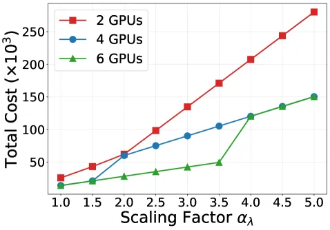
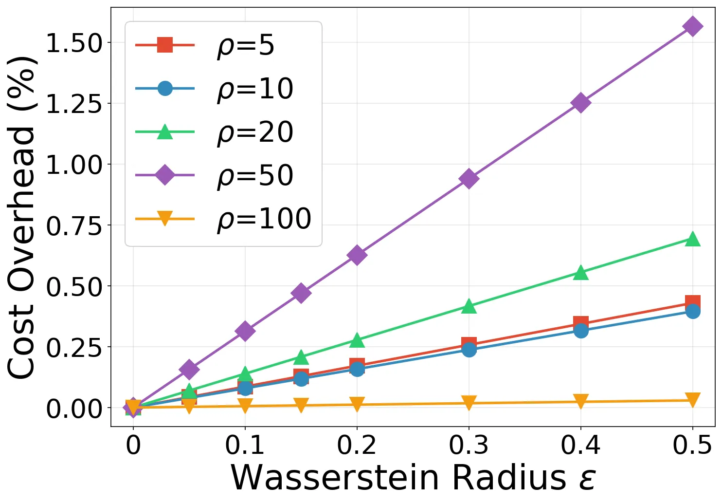
• Wasserstein 鲁棒性增加适度 premium（即使 $\varepsilon=0.5$ 也 $< 1.3\%$ overhead）
• overhead 随 $\rho$ 增长，因为更高的 cost ratio 放大 DRO regularization term
• 实践中 $\varepsilon \in [0.1, 0.2]$ 提供鲁棒性且 $< 0.5\%$ overhead

Distribution Shift Robustness

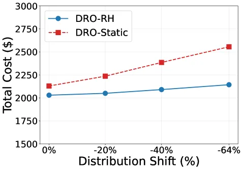
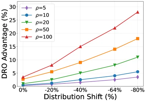
关键发现：

• Static 策略在分布漂移下性能退化，而 rolling horizon 通过周期性 re-optimization 保持鲁棒性
• DRO advantage 随 shift magnitude 单调增长
• SAA 在 training trace 上略优但在 shifted workloads 上显著退化
• Fig. 6 显示 gap 随 $s$ 增大：SAA 的 P99 从 3.0s 增至 ~18s，而 DRO 仅增至 ~9s @ $s=3.0$

Ablation Study（Table V）

Variant	Cost	P99 (s)	Goodput	SLO viol.(%)
BCD-DRO (ours)	13,476 ± 208	8.12 ± 0.65	5.01 ± 0.25	26.4 ± 3.7
− Routing (uniform π)	93,878 ± 5,152	177.62 ± 11.90	0.63 ± 0.06	93.8 ± 0.6
− DRO (SAA)	24,864 ± 1,534	11.02 ± 1.55	3.68 ± 0.35	45.8 ± 5.2
− Prefix caching (δ=0)	13,476 ± 208	9.95 ± 1.29	4.39 ± 0.37	35.4 ± 5.4

关键发现：

• 禁用 routing optimization 导致 cost 增加 7x，goodput 下降 42x
• SAA 相比 DRO cost 增加 85%，SLO violation 增加 246%
• 禁用 prefix caching 使 P99 延迟增加 22%

Secondary Weights Sensitivity（Figure 4）

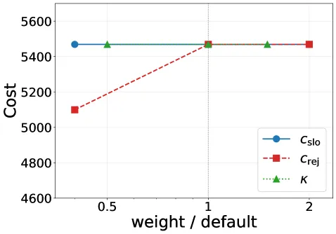
操作点在 $c_{\text{slo}}$ 和 $c_{\text{rej}}$ 变化 5× 范围内保持稳定，仅 $c_{\text{rej}}$ 减半时 shed 最贵 class。reservation quantile $q^* \approx 91\%$ 保持不变。

Key Takeaway 3： Wasserstein 鲁棒性和 rolling-horizon adaptation 解决工作负载漂移的互补方面：歧义集保护 against model mismatch，周期性 re-optimization 跟踪 live workload distribution 的时序变化。

七、相关工作

Table I: Related Work Comparison

System	Memory Layout	Reservation Policy	Joint Optimization	Length Uncertainty Handling	Robustness Guarantee
PagedAttn/vLLM [1]	paged	reactive	–	none	–
Orca [2]	cont. batch	–	–	none	–
DistServe [24]	P/D split	–	topology	none	–
Sarathi-Serve [3]	chunked	–	–	none	–
H2O [4], SnapKV [5]	eviction	–	–	post-hoc	–
Length predictors	any	point est.	–	regression	–
BCD-DRO (ours)	any	DRO-opt.	✓	Wasserstein	Wasserstein

LLM Serving Systems

• vLLM、Orca、DistServe、Sarathi-Serve 等通过不同的 memory layout 策略（paged attention、continuous batching、P/D split、chunked prefill）提高 throughput
• H2O、SnapKV 通过 dynamic eviction 管理 KV cache
• 这些方法都是 reactive 的，没有显式处理 output length uncertainty

KV Cache Management for RL

• ReMAX、CoCa 等通过 early exit 或 speculative decoding 减少 rollout 长度
• WAR 的 SuffixDecoding 与此方向正交且互补

Distributionally Robust Optimization

• DRO 已在 finance、supply chain 等领域广泛应用
• 本文首次将 Wasserstein DRO 引入 LLM serving 的 KV cache management

八、局限性

1. 仿真评估：结果基于 trace-driven simulation，尚未在真实 production system 上验证
2. 模型规模限制：仅在 70B 模型上评估，更大/更小模型的泛化性待验证
3. 成本参数敏感性：虽然对 secondary weights 鲁棒，但 cost ratio $\rho$ 的选择仍需要领域知识
4. Re-optimization 频率：周期性 re-optimization 的频率选择缺乏理论指导
5. 扩展性：当 $|\mathcal{I}| \geq 20, N \geq 5000$ 时 BCD-DRO 求解时间可能超出 practical 窗口

九、未来方向

1. Production runtime integration：集成到 vLLM、SGLang 等生产级 serving runtime
2. Online adaptation：使用 streaming workload statistics 进行在线适应
3. Energy-aware scheduling：联合优化 with energy-aware and geographically distributed inference scheduling
4. Learned cost parameters：从历史数据中学习最优 cost ratio $\rho$
5. Multi-model support：适配不同规模 LLM 的 KV cache 管理

十、总结

核心贡献

1. 联合优化框架：BCD-DRO 联合优化 GPU 并行配置、KV cache 预留、请求路由和前缀缓存，是唯一 co-optimize 所有四个 control knobs 的方法
2. Wasserstein DRO 形式化：首次将 KV cache 预留建模为 Wasserstein DRO 问题，提供 distribution shift 的显式保护
3. Critical fractile 结构：推导出 closed-form 最优预留策略 $r_i^* = L_{\text{in}}^i + F_i^{-1}(\rho/(\rho+1))$，自动适应 cost regime
4. 可扩展算法：BCD-DRO 分解算法在 production-scale 实例上可行，而 monolithic MIBLP solver 失败
5. 显著性能提升：最高 56% 成本降低，同时保持竞争性 P99 延迟和 goodput

关键实验结论

• DRO 是唯一在整个 $\rho \in \{2, 10, 100\}$ 范围保持 bounded cost 的方法
• Real-time 场景（$\rho=100$）下 DRO 比 P90 基线低 56% 成本
• BCD-DRO 在 48-GPU cluster 上 257.7s 收敛，而 MIBLP 在小规模即 timeout
• 禁用 routing optimization 导致 cost 增加 7x
• SAA 在 distribution shift 下显著退化，DRO 保持鲁棒

附图索引

编号	文件名	说明
Figure 1	figures/wildcard-match/figure-1-system-model.png	BCD-DRO 系统模型：control plane + data plane 架构
Figure 2a	figures/wildcard-match/figure-2-cost-vs-ratio.png	Cost vs cost ratio ρ
Figure 2b	figures/wildcard-match/figure-2-dro-quantile.png	DRO quantile vs theoretical q*
Figure 3a	figures/wildcard-match/figure-3-arrival-scaling.png	Cost vs arrival rate scaling
Figure 3b	figures/wildcard-match/figure-3-epsilon-sensitivity.png	Cost overhead vs Wasserstein radius ε
Figure 4	figures/wildcard-match/figure-4-secondary-weights.png	Secondary weights sensitivity (cost + P99 latency)
Figure 5a	figures/wildcard-match/figure-5-static-vs-rolling.png	Static vs rolling horizon
Figure 5b	figures/wildcard-match/figure-5-dro-advantage.png	DRO advantage vs ρ and shift magnitude
Figure 6	figures/wildcard-match/figure-6-bcd-dro-vs-saa.png	BCD-DRO vs SAA under distribution shift

附表格索引

编号	说明
Table I	Related work comparison：System vs Mem. Res. Joint Len. Robust.
Table II	DRO vs baselines across application scenarios (ρ ∈ {2, 5, 10, 20, 50, 100})
Table III	Algorithm scalability：MIBLP vs BCD-DRO solve time vs problem size
Table IV	Cost across three cost-ratio regimes (ρ ∈ {2, 10, 100})
Table V	Ablation on heterogeneous instance：routing/SAA/prefix-caching ablation